Aligning Latent Geometry for Spherical Flow Matching

Linear vs. spherical transport

Latent flow matching usually connects Gaussian noise to a VAE latent with a Euclidean chord. Both endpoints concentrate in thin spherical shells, so the chord cuts through radii that neither endpoint naturally occupies. The fix is to put both endpoints on the same token-wise sphere and train along the spherical arc.

t 0.00

Loading linear path...

1. Linear interpolation. Samples occupy a thin shell, while the straight chord between noise and data moves through the interior.

Loading spherical path...

2. Projected spherical interpolation. The same samples are radially projected to one radius and connected by slerp.

3. Norm distance. Linear transport moves away from the fixed-radius shell; slerp stays at distance zero.

4. Radial share. Linear targets contain radial motion; slerp targets are tangent to the sphere.

Empirical measurements

01

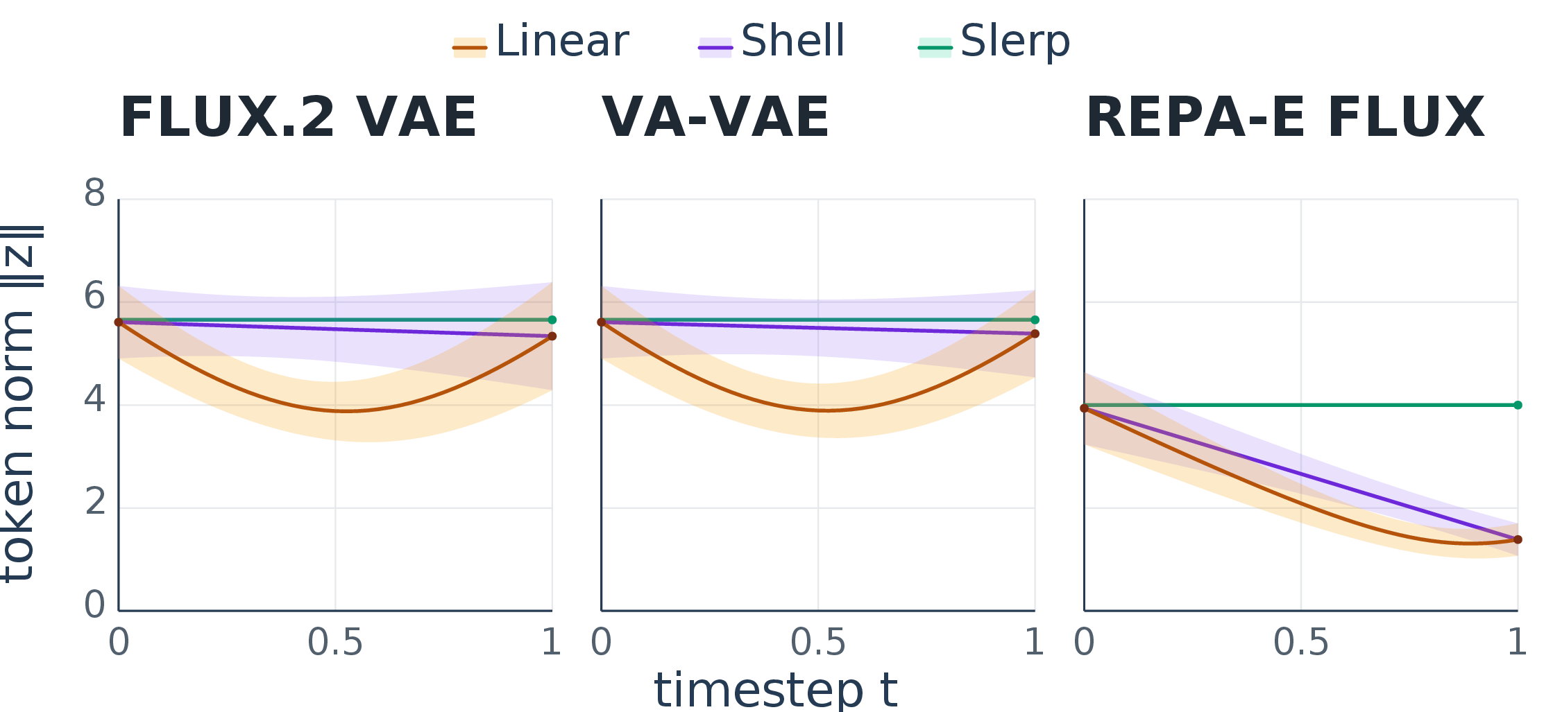
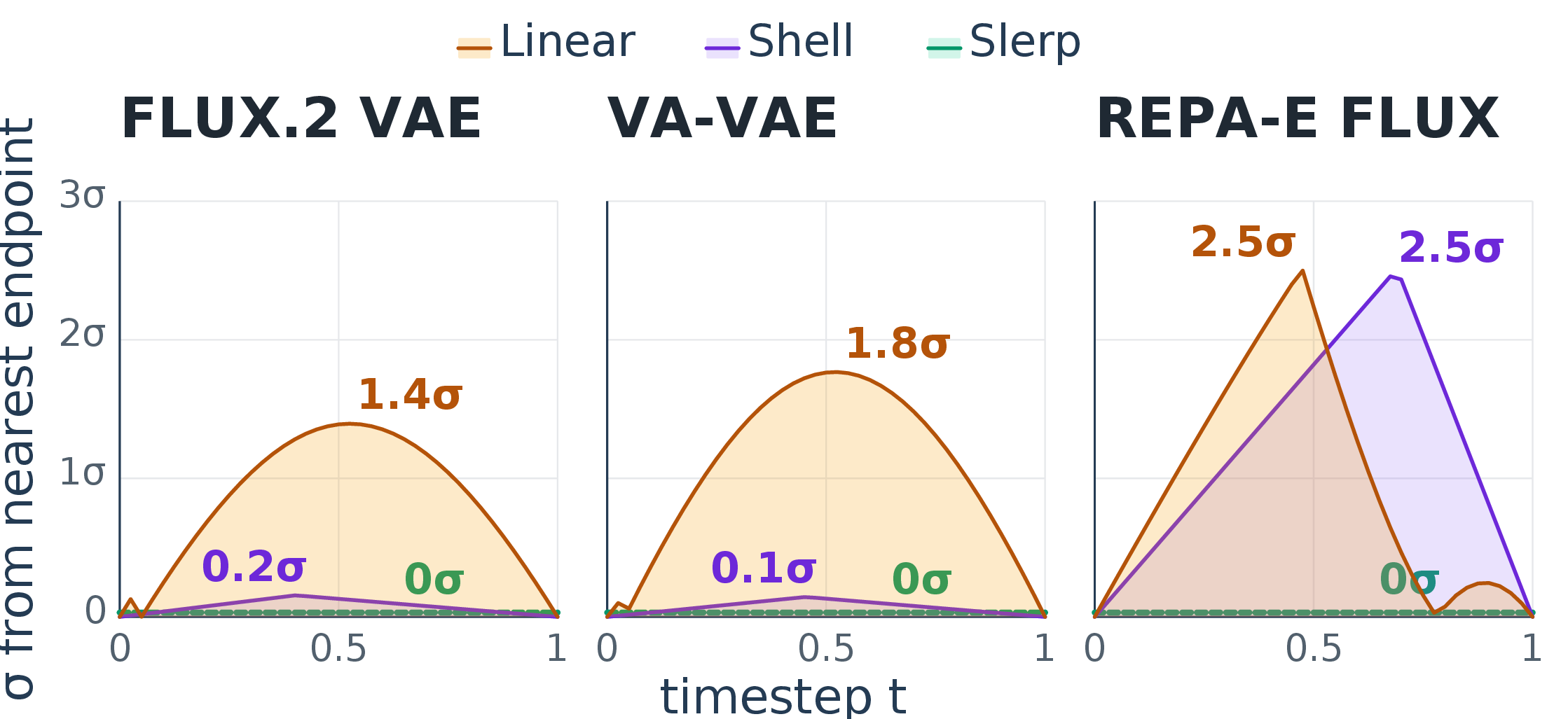
Linear paths leave the latent support.

Per-token norms concentrate tightly across all three tokenizers (\(\text{CV} \le 0.23\)). After preprocessing, FLUX.2 and VA-VAE sit close to the Gaussian shell (\(\bar r/\sqrt d = 0.94\) and \(0.95\)), while REPA-E FLUX.1 sits well below it (\(\bar r/\sqrt d = 0.35\)). Projection puts every token at \(\sqrt d\). Linear paths then deviate up to \(1.4\sigma\), \(1.8\sigma\), and \(2.5\sigma\) from the nearest endpoint shell; slerp stays on the fixed radius throughout the flow.

Per-token latent norms along linear, shell, and spherical-slerp paths for three tokenizers — Per-token norm along linear, shell, and slerp paths for representative tokenizers. Lines average 2048 pairs; bands show \(\pm 1\sigma\); the horizontal reference is the fixed spherical radius.

Off-shell distance in standard deviations for linear, shell, and spherical-slerp paths — Off-shell distance for each path, in standard deviations from the nearest endpoint shell. Larger values indicate latent regions rarely occupied by either endpoint; slerp remains at the fixed spherical radius.

02

Direction carries content.

Keeping the anchor direction (radius swapped to a same-class neighbor) leaves the decoded image close to the anchor, whereas keeping the anchor radius (direction swapped) moves it almost as far as replacing the whole latent with the neighbor — an asymmetry visible on both LPIPS and DINOv2 distances. The decoder is much more sensitive to direction than to radius.

Anchor original latent

Anchor direction + neighbor radius

Anchor radius + neighbor direction

Neighbor same-class latent

FLUX.2 decoder, same-class swaps (paper Fig. 5). Highlighted pair = matched percept.

03

Linear targets waste radial budget.

Linear flow matching allocates substantial supervision to radial motion, a component to which the decoder is less sensitive. Decomposing the per-token velocity target into radial and tangential components yields an endpoint-dependent radial share — about 50% at both endpoints for FLUX.2 and VA-VAE, and reaching about 90% at the noise endpoint for REPA-E FLUX.1, whose data shell radius falls farthest below \(\sqrt d\). Slerp on the sphere makes it identically zero by construction.

Radial energy share of flow matching velocity targets — Radial share for linear paths versus spherical slerp.

Watch the radial component appear.

Filled marker, linear chord: the gray velocity \(u\) splits into a radial part (red, wasted on changing norm) and a tangential part (blue, useful for changing direction). Open marker, slerp arc: the velocity \(v_{\text{slerp}}\) is tangent to the sphere by construction — no radial waste arises.

radial share

0%

Spherical flow matching

Building a spherical support — token projection, decoder/discriminator finetuning, and drawing noise on the same sphere — already closes most of the gap with vanilla linear flow matching. Replacing the chord with the slerp geodesic on top gives the best observed trajectory. The diffusion architecture and conditioning stay unchanged.

1

Project tokens to a fixed radius.

\(z_{i,j} \leftarrow \sqrt d \cdot z_{i,j} / \|z_{i,j}\|\). The encoder stays frozen; the decoder and discriminator are finetuned to decode projected latents.

2

Sample noise on the same sphere.

Draw \(\epsilon \sim \mathcal N(0, I_d)\), then use \(z_0 = \sqrt d\,\epsilon/\|\epsilon\|\). This keeps the angular part of the Gaussian prior.

3

Train along slerp.

Replace the chord with the geodesic arc and project the predicted velocity onto the tangent space; integrate with the exponential map at inference so samples stay on the sphere. SiT architecture and conditioning stay unchanged — no auxiliary encoder, no representation-alignment objective.

FID training curves comparing vanilla linear, shell, spherical linear, and spherical slerp transport — Spherical support gives most of the gain; the tangent slerp path gives the best trajectory.

ImageNet-256 results

FLUX.2 B/2, CFG 1.0

26.14 -> 20.21 22.7% lower FID

VA-VAE B/1, CFG 1.5

10.86 -> 7.81 28.1% lower FID

REPA-E FLUX.1 B/2, CFG 1.5

13.83 -> 6.88 50.2% lower FID

FLUX.2 B/2, 200 epochs

3.22 -> 2.91 CFG 1.5 FID

Tokenizer	Scale	CFG	Linear FID	Slerp FID	Relative change
FLUX.2	B/2	1.0	26.14	20.21	-22.7%
FLUX.2	XL/2	1.5	4.32	3.95	-8.6%
VA-VAE	B/1	1.5	10.86	7.81	-28.1%
REPA-E FLUX.1	B/2	1.5	13.83	6.88	-50.2%

Reconstructions and component swaps

One representative reconstruction panel and one component-swap panel are shown here. The repeated tokenizer variants are kept out of the page to reduce visual clutter.

FLUX.2 reconstruction comparison: original, finetuned vanilla, and spherical — FLUX.2 reconstruction: original / finetuned vanilla / spherical. The reconstructions are visually near-identical; generation quality depends on the latent geometry.

FLUX.2 same-class component swap grid — FLUX.2 component swap: direction-versus-radius pattern.

ImageNet sample: Chesapeake Bay retriever

BibTeX

@article{meral2026aligning,
  title={Aligning Latent Geometry for Spherical Flow Matching in Image Generation},
  author={Meral, Tuna Han Salih and Oktay, Kaan and Yesiltepe, Hidir and Akan, Adil Kaan and Yanardag, Pinar},
  journal={arXiv preprint arXiv:2605.15193},
  year={2026}
}